最短路

Posted on 2022-12-03 In Data Structure and Algorithm

最短路

Floyd

定义数组f[k][x][y]，表示只允许经过1到k时x到y的最短路长度。

for (k = 1; k <= n; k++) {
  for (x = 1; x <= n; x++) {
    for (y = 1; y <= n; y++) {
      f[k][x][y] = min(f[k - 1][x][y], f[k - 1][x][k] + f[k - 1][k][y]);
    }
  }
}

然而时间复杂度为 \(O(n^3)\)。

Dijkstra

只能解决非负权图。

将结点分为两个集合：已经确定最短路长度的集合，和未确定的集合。

初始化 \(dis[start]=0\)，其他为 \(+\infty\)

随后重复：

取出未确定的集合中最短路长度最小的结点加入到确定的集合中
更新结点的最短路长度

void dijkstra(){
    memset(dis, INT_MAX, sizeof(dis));
    memset(vis, 0, sizeof(vis));
    dis[start] = 0;
    for(int i = 1; i <= n; i++){
        int mindis = INT_MAX;
        int pos = 0;
        for(int j = 1; j <= n; j++){
            if(!vis[j] && dis[j] < mindis){
                pos = j;
                mindis = dis[j];
            }
        }
        if(pos != 0){
            vis[pos] = 1;
            for(int j = 1; j <= n; j++){
                dis[j] = min(dis[j], dis[pos] + graph[pos][j]);
            }
        }
    }
}

还可以使用优先队列，时间复杂度为 \(O(m\log m)\)

struct node{
    int dis;
    int u;
    bool operator>(const node& a){
        return dis > a.dis;
    }
};

void dijkstra(){
    memset(dis, INT_MAX, sizeof(dis));
    memset(vis, 0, sizeof(vis));
    dis[start] = 0;
    std::priority_queue<node, vector<node>, greater<node>> q;
    int d = 0;
    node nd;
    nd.dis = 0;
    nd.u = start;
    q.push(nd);
    while(!q.empty()){
        int u = q.top().u;
        q.pop();
        if(vis[u]){
            continue;
        }
        vis[u] = 1;
        for(int i = 1; i <= n; i++){
            if(dis[i] > dis[u] + graph[u][i]){
                dis[i] = dis[u] + graph[u][i];
                node tmp;
                tmp.u = i;
                tmp.dis = dis[i];
                q.push(tmp);
            }
        }
    }
}

计组实验1

Posted on 2022-11-21 Edited on 2022-12-20 In Computer Organization

单周期CPU

RV32I指令集

lui:

\(x[rd] = sext(immediate[31:12] << 12)\)

auipc:

\(x[rd] = pc + sext(immediate[31:12] << 12)\)

一些csr相关的，在lab2中用到：

csrrw:

csrrw rd,offset,rs1

\(t = CSRs[csr]; CSRs[csr] = x[rs1]; x[rd] = t\)

csrrs:

csrrs rd,offset,rs1

Any bit that is high in rs1 will cause the corresponding bit to be set in the CSR, if that CSR bit is writable. Other bits in the CSR are unaffected (though CSRs might have side effects when written).

\(t = CSRs[csr]; CSRs[csr] = t \or x[rs1]; x[rd] = t\)

csrrc:

csrrc rd,offset,rs1

Any bit that is high in rs1 will cause the corresponding bit to be cleared in the CSR, if that CSR bit is writable. Other bits in the CSR are unaffected.

\(t = CSRs[csr]; CSRs[csr] = t \land ∼x[rs1]; x[rd] = t\)

取指

取出PC地址的指令
修改PC的值
- 若跳转，修改为跳转地址
- 否则改为PC+4

when(io.instruction_valid) {
  io.instruction := io.instruction_read_data
  // lab1(InstructionFetch)
  io.instruction_address := pc
  when(io.jump_flag_id){
    pc := io.jump_address_id
  }.otherwise{}
    pc := pc + 4.U
  }
  // la1(InstructionFetch) end


}.otherwise{
  pc := pc
  io.instruction := 0x00000013.U
}
io.instruction_address := pc

译码

控制信号：

ALUOp1Src: 控制ALU第一个输入为指令地址或寄存器
ALUOp2Src: 控制ALU第二个输入为寄存器或立即数，R指令取0
MemoryRE: 内存读使能，Load指令取1
MemoryWE: 内存写使能，Store指令取1
RegWE: 寄存器写使能，R, I, L, auipc, lui, jal, jalr
RegWriteSrc: 寄存器写回数据来源，L选择内存，jal, jalr选择指令地址，其他选择ALU计算结果

执行

进行ALU运算
判断是否跳转


alu.io.op1 := Mux(
  io.aluop1_source === ALUOp1Source.Register,
  io.reg1_data,
  io.instruction_address
)
alu.io.op2 := Mux(
  io.aluop2_source === ALUOp2Source.Immediate,
  io.immediate,
  io.reg2_data
)

io.if_jump_flag := opcode === Instructions.jal ||
  (opcode === Instructions.jalr) ||
  (opcode === InstructionTypes.B) && MuxLookup(
    funct3,
    false.B,
    IndexedSeq(
      InstructionsTypeB.beq -> (io.reg1_data === io.reg2_data),
      InstructionsTypeB.bne -> (io.reg1_data =/= io.reg2_data),
      InstructionsTypeB.blt -> (io.reg1_data.asSInt < io.reg2_data.asSInt),
      InstructionsTypeB.bge -> (io.reg1_data.asSInt >= io.reg2_data.asSInt),
      InstructionsTypeB.bltu -> (io.reg1_data.asUInt < io.reg2_data.asUInt),
      InstructionsTypeB.bgeu -> (io.reg1_data.asUInt >= io.reg2_data.asUInt)
    )
  )
io.if_jump_address := io.immediate + Mux(opcode === Instructions.jalr, io.reg1_data, io.instruction_address)

访存

读内存，判断是lb, lbu, lh, lhu, lw，根据不同指令取不同位数
写内存，根据不同指令取不同位数

写回

没什么好说的。

二叉树遍历

Posted on 2022-11-13 In Data Structure and Algorithm

二叉树遍历

struct Node{
    int data;
    Node* lchild;
    Node* rchild;
};
typedef Node* BiTree;

先序遍历

void preorder(BiTree T){
    if(T == NULL){
        return;
    }
    visit(T);
    preorder(T->lchild);
    preorder(T->rchild);
}

void preorder(BiTree T){
    if(T == NULL){
        return;
    }
    std::stack<BiTree> st;
    st.push(T);
    BiTree p;
    while(!st.empty()){
        p = st.top();
        st.pop();
        visit(p);
        if(p->rchild != NULL){
            st.push(p->rchild);
        }
        if(p->lchild != NULL){
            st.push(p->rchild);
        }//先进右再进左
    }
}

中序遍历

void inorder(BiTree T){
    if(T == NULL){
        return;
    }
    inorder(T->lchild);
    visit(T);
    inorder(T->rchild);
}

void inorder(BiTree T){
    if(T == NULL){
        return;
    }
    std::tack<BiTree> st;
    BiTree p = T;
    while(p != NULL || !st.empty()){
        while(p != NULL){
            st.push(p);
            p = p->lchild;
        }//一直向左
        p = st.top();
        st.pop();
        visit(p);
        p = p->rchild;
    }
    
}

后序遍历

void postorder(){
    if(T == NULL){
        return;
    }
    postorder(p->lchild);
    postorder(p->rchild);
    visit(p);
}

void postorder(){
	if(T == NULL){
        return;
    }
    std::stack<BiTree> st;
    BiTree p = T, r = NULL;
    while(p != NULL || !st.empty()){
        while(p != NULL){
            st.push(p);
            p = p->lchild;
        }
        p = st.top();
        if(p->rchild == NULL || r == p->rchild){
            st.pop();
            visit(p);
            r = p;
            p = NULL;
        }
        else{
            p = p->rchild;
        }
    }
}

层次遍历

void levelorder(BiTree T){
    if(T == NULL){
        return;
    }
    queue<BiTree> q;
    q.push(T);
    BiTree p;
    while(!q.empty()){
        p = q.front();
        q.pop();
        visit(p);
        if(p->lchild != NULL){
            q.push(p->lchild);
        }
        if(p->rchild != NULL){
            q.push(q->rchild);
        }
    }
}

根据先序和中序构建二叉树

void construct(Node* root, int* pre, int* mid, int l1, int r1, int l2, int r2){
	if(l1 > r1)return;
	root->data = pre[l1];
	int pos = 0;
	for(int i=l2;i<=r2;i++){
		if(pre[l1] == mid[i]){
			pos = i;
			break;
		}
	}// 找到根结点在中序序列中的位置
	if(pos>l2){// 构造左子树
		root->left = new Node();
		construct(root->left, pre, mid, l1 + 1, l1 + pos - l2, l2, pos - 1 );
	}
	if(pos<r2){// 构造右子树
		root->right = new Node();
		construct(root->right, pre, mid, l1 - l2 + pos + 1, r1, pos + 1, r2);
	}
}

ML chapter1

Posted on 2022-11-11 Edited on 2023-07-11 In Artificial Intelligence

Polynomial Curve Fitting

\[ y(x,\vec w) = w_0 + w_1x + w_2x^2+\cdots+w_Mx_M = \displaystyle\sum_{j=0}^{M}w_jx^j \] minimize an error function that measures the misfit between the function \(y\).

One simple choice of error function, which is widely used, is given by the sum of the squares of the errors between the predictions \(y(x_n, \vec w)\) for each data point \(x_n\) and the corresponding target values \(t_n\) : \[ E(\vec w) = \dfrac{1}{2}\displaystyle\sum_{n=1}^{N}[y(x,\vec w)-t_n]^2 \]

find \(\vec w^\star\) such that \(E(\vec w)\) is as small as possible.

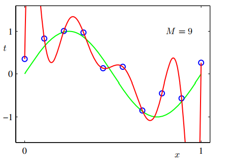
choose \(M\) : model comparison or model selection

overfitting:

RMS: \[ E_{RMS} = \sqrt{2E(\vec w^\star)/N} \] By adopting a Bayesian approach, the over-fitting problem can be avoided.

Indeed, in a Bayesian model the effective number of parameters adapts automatically to the size of the data set.

regularization
\[ \tilde{E}(\vec w)= \dfrac{1}{2}\displaystyle\sum_{n=1}^{N}[y(x,\vec w)-t_n]^2 + \dfrac{\lambda}{2}\lVert\vec w\rVert^2 \] the coefficient \(\lambda\) governs the relative importance of the regularization term compared with the sum-of-squares error term.

Also known as ridge regression.

Bayesian Probabilities

\[ p(\mathbf {w}|\mathcal{D})=\dfrac{p(\mathcal{D}|\mathbf w)p(\mathbf w)}{p(\mathcal D)} \]

\[ p(\mathcal D) = \int p(\mathcal{D}|\mathbf w)p(\mathbf w)\mathrm d \mathbf w \]

\[ \text{posterprior}\varpropto \text{likelihood}\times \text{prior} \] Maximum Likelihood : choose \(\mathbf w\) to maximize \(p(\mathcal D|\mathbf w)\), error function with negative log.

并查集

Posted on 2022-11-10 Edited on 2022-12-01 In Data Structure and Algorithm

并查集

并查集：实现为森林，其中每个树表示一个集合。

合并：合并对应的集合（合并树）
查询：查询元素所在集合（查询元素对应根结点）

1	std::vector<int> f;

查询：沿着树向上，直到根结点。

1
2
3

int find(int x){
    return x == f[x] ? x : find(f[x]);
}

路径压缩

直接连至根结点。

1
2
3

int find(int x){
    return x == f[x] ? x : f[x] = find(f[x]);
}

合并

1
2
3

void unite(int x, int y){
    f[find(x)] = find(y);
}

启发式合并

合并时将节点较少，或深度较小的连另一棵。

void unite(int x, int y){
    x = find(x);
    y = find(y);
    if(x == y){
        return;
    }
    if(size[x] < size[y]){
        swap(x, y);
    }
    f[y] = x;
    size[x] += size[y];
}

删除

删除叶子节点，只需将其父亲设为自己。

void erase(int x){
    size[find(x)]--;
    find(x) = x;
}

移动

void move(int x, int y){
    int fx = find(x), fy = find(y);
    if(fx == fy){
        return;
    }
    f[x] = fy;
    size[fx]--;
    size[fy]++;
}

应用：Kruskal算法

为了构造一棵最小生成树（森林），每次都选取最小边权的边，若加入此边后产生环则删去，直到加入了\(n-1\)条边。

换句话说，就是维护一堆集合，合并集合。

struct edge{
  int u; int v; int w;
}e[50];

bool cmp(edge a, edge b){
    return a.w < b.w;
}

// n vertex, m edges, construct forest
int kruskal(){
    sort(e, e + m, cmp);
    for (int i = 0; i <= n;i++){
        f[i] = i;
    }
    int ans = 0;
    int cnt = 0;
    for (int i = 0; i < m;i++){
        int u = e[i].u;
        int v = e[i].v;
        int d = e[i].d;
        u = find(u);
        v = find(v);
        if(u != v){
            f[u] = v;
            ans += d;
            cnt++;
        }
    }
    return ans;
}